%%{init: {"theme": "base", "themeVariables": {"primaryColor": "#E8ECFF", "primaryBorderColor": "#4054B2", "primaryTextColor": "#16171B", "lineColor": "#3B4351", "edgeLabelBackground": "#FAF7F0", "clusterBkg": "#EFE9DC", "clusterBorder": "#766F65"}, "flowchart": {"rankSpacing": 28, "nodeSpacing": 42, "subGraphTitleMargin": {"top": 4, "bottom": 14}}}}%%
flowchart TB
    HUM["Human labels · stratified, per task type"]
    subgraph DEV["Development loop"]
        direction TB
        SUT["System under test"]
        DJ(["Development judge"])
        SUT --> DJ
        DJ -->|"consulted hourly"| SUT
    end
    FRZ(["freeze · snapshot<br/>the final system"])
    subgraph EV["Held-out evaluation"]
        direction TB
        EJ(["Evaluation judge<br/>development never sees it"])
        REP["Reported result"]
        XT["✗"]
        EJ --> REP
        EJ -.->|"no tuning feedback"| XT
    end
    SUT -->|"final system"| FRZ
    FRZ -->|"fresh outputs"| EJ
    HUM -.->|"calibrate"| DJ
    HUM -.->|"calibrate"| EJ
    classDef gate fill:#F7E6B5,stroke:#8A5A00,color:#16171B
    classDef world fill:#EFE9DC,stroke:#766F65,color:#16171B
    classDef risk fill:#F4D7D5,stroke:#A4161A,color:#16171B
    class FRZ gate
    class HUM world
    class XT risk
24 Evaluation and Experimental Method
Chapter 23 left one question standing, and it is the expensive one. The team demos beautifully; the engineers who built it believe in it; the transcript reads like a well-run meeting, the dashboard is green, and the invoice is four times what a single agent would have cost. Is it better? Around that innocent word an entire discipline hangs, because in this field the question is routinely answered by anecdote, adrenaline, and comparison with an opponent assembled principally to lose — the lone model with no tools, no iteration, and a prompt written by someone rooting for the other side. The preface warned that you cannot unit-test a vibe; this chapter is about what you can do instead, and it is a great deal more than the field’s current habits suggest.
The honest answer is hard to obtain for reasons that deserve respect rather than shortcuts. The system is stochastic, so a single run is an anecdote and the same configuration will beat itself on Tuesdays. The tasks are long-horizon, so errors compound and metrics measured mid-way mislead. The workers are plural, so when quality moves nobody knows which agent moved it. Every sample costs real money, so the statistics must be done on a budget that would make an agronomist laugh. And the substrate will not hold still: the model under everything upgrades on a vendor’s schedule, and this quarter’s improvement may belong to the provider rather than to you. Evaluation under these conditions is not quality assurance with extra steps; it is experimental method — the discipline agriculture and medicine spent a century learning, arriving at software that argues back.
The book’s contribution to the problem is that its systems have been building the instruments all along. The journal — the append-only event record that Section 20.3 made the runtime’s single source of truth — holds every decision with its full context; Chapter 23‘s replay makes any incident a deterministic test; the incident suite is an evaluation set growing itself from production; and the trace-annotation method behind the MAST taxonomy shows what disciplined reading of such records looks like at scale. The classical multi-agent community, meanwhile, supplies a working example of benchmarking culture — standardised simulators, controlled comparisons, results that replicate — that the language-model world has yet to import. And over the whole chapter stands the emphasis the preface promised: the baseline. Chapter 1 gave you a framework for deciding whether to build a team at all; this chapter is that judgement call handed instruments, and the instruments’ first duty is to keep the comparison honest.
The sections follow the evaluator’s questions in the order they arise. What, exactly, is the comparison — and how strong must the opponent be before winning means anything (Section 24.1)? What is the measure — outcomes, process, cost, and robustness, and what to do where ground truth runs out (Section 24.2)? Who grades open-ended work — the judge problem, in which the marker is a model with biases of its own and, on a bad day, a conflict of interest (Section 24.3)? What changes when a person is not the grader but part of the graded unit — the human inside the measurement, and the older sciences’ rules for measuring people (Section 24.4)? How many runs make a fact, and how does one find out which agent earns its keep (Section 24.5)? And against what suite, maintained how, for how long — benchmarks, their decay, and the living evaluation distilled from your own traffic (Section 24.6)? At the end the system will be measured, compared, and honestly accounted — good today, against these tasks, on this substrate. What an adversary can make it do tomorrow is another matter, and the next chapter’s.
24.1 The Question, and the Opponent Built to Lose
“Is it better?” is not yet a question; it is a question-shaped noise with two blanks in it. Better than what — and at what cost? Evaluation of a multi-agent system is never absolute, because nobody deploys a system against nothing: the alternative is always something — a single agent, a pipeline, the intern, the status quo — and the only claim worth making is comparative, against the alternative you would actually build instead. The cost blank is not an accounting afterthought but half the verdict: a team that scores 5% higher at four times the price has not won an argument; it has stated a trade, and whether the trade is good depends on facts about your task — how much a marginal point of quality is worth, and to whom — that no benchmark knows. Fill in both blanks and “is it better?” becomes answerable. Leave them blank and any answer will do, which is, not coincidentally, how the field’s weakest claims are constructed.
The commonest failure is the one the section title names: the opponent built to lose. It is rarely fraud; it is enthusiasm plus asymmetric effort. The team gets six weeks of prompt-tuning, hand-picked tools, an iteration loop, and a champion who stays late; the baseline gets an afternoon, a default prompt, and nobody’s love. Then the comparisons come out, and the paper — or the pitch deck — reports that the team wins. The riggings are worth learning to spot because most are invisible in the headline: the baseline ran a weaker model (the team on the frontier model, the “single agent” on something cheaper); the baseline was denied the tools the team’s members each enjoy; the baseline was denied iteration (one shot, against a team that critiques and revises for twenty turns); the baseline was denied the budget (a fraction of the tokens, then judged on quality alone as though the tokens were free). A result of this shape does not show that the team beats an agent; it shows that effort beats neglect — a finding of no great novelty. Chapter 14’s audit of the debate literature met the same pattern from the other side: reported gains that shrink, sometimes to nothing, when the single-model baseline is given the same compute and a competent prompt.
So the discipline is to specify the honest opponents in advance, and the book’s own distinctions say what they are. The first is the strong single agent: the same frontier model, the same tools, the same token budget — all of it, the full multiple the team would spend, available as iteration, self-critique, retries, and self-consistency — in one context, with no coordination losses, no summarisation hops, and no whisper game, because there is nobody to whisper to. One exclusion must be stated in the protocol, because it looks like a rigging and is in fact the experiment: “the same tools” does not include a tool that spawns subagents. Delegation is the variable under test — the moment the baseline can hire ephemeral workers it stops being the control arm and becomes Section 1.3.6’s delegating single agent, a third architecture, worth an arm of its own wherever it is the incumbent — so the line is drawn at the locus of control: one context, one journal, everything else equal. Chapter 21 taught why this opponent is formidable: everything the team pays in joins, the single agent keeps. The second is the fixed workflow, Chapter 1’s most practically important look-alike: the predetermined pipeline with model calls at fixed points — cheap, deterministic, testable, and very often sufficient, since, as Chapter 19 put it, most tasks need less topology than the showcases suggest. And both opponents deserve what the team had: a champion. The evaluation is honest when someone competent has genuinely tried to make each alternative win — adversarial assignment, the same instinct Chapter 14 institutionalised in the critic, now applied to the experiment itself.
What does an honest result look like once the opponents are real? The book has been citing one all along — a vendor’s account of its own system, cited here for the shape of the claim rather than for a referee’s stamp it never had. Anthropic’s evaluation of its research system reported a genuine win for the orchestrator over a strong single agent — and reported, in the same breath, the price (many times the tokens) and the boundary (tasks that parallelise across independent facets; tasks that fit one context showed no such gain) (2025). That triple — better at this class of task, at this cost, and not elsewhere — is the canonical shape of a defensible claim, and its third clause is the one enthusiasm always omits: every honest evaluation delimits its own domain of validity, because a system evaluated on research synthesis has been evaluated on nothing else, and the reader who deploys it on contract review has left the evidence behind.
All of which turns Chapter 1’s decision framework from a judgement call into an experiment. The questions asked there in the armchair — does the task genuinely decompose, do the objectives genuinely diverge, does one context suffice — were answered, in good faith but a priori, by inspection; the lab answers them a posteriori, with instruments. Build all three systems — the team, the strong single agent, the workflow; run them on the same task set, many times each; record everything, because the journal makes recording free. That triple experiment is this chapter’s running spine, with the case-study’s coding team as the defendant — and before it can run, one question must be settled that sounds trivial and is not: what gets written down? Outcomes are the obvious answer, and they are perhaps a quarter of it.
24.2 What to Measure: Outcomes, Process, Cost, Robustness
The seduction to resist is the single number. Leaderboard culture runs on one score per system, and one score is precisely what a multi-agent evaluation cannot afford, because the reduction discards the two things that make the exercise multi-agent at all: how the agents worked together, and what the working-together cost. A complete record answers four questions — did it succeed, how did it get there, at what price, and how much does the answer wobble — and the four families of metrics that follow are those questions made operational. The good news is a Chapter 23 dividend: all four are views over the journal, so the marginal cost of measuring everything is close to nothing, and the experimental instrumentation was installed the day the runtime was built. Measurement, on this architecture, is not something added to the system; it is something asked of the record.
| Family | Question it answers | What you measure | Where the number comes from |
|---|---|---|---|
| Outcomes | Did it succeed? | Pass/fail against ground truth; rubric clauses for open-ended quality | Executable truth, human labels, or downstream acceptance |
| Process | How did it get there? | Duplicated work per task, messages per resolution, conflict and escalation rates, dead-letter counts, idle time, the divergence signatures of Chapter 21’s failure catalogue | Views over the journal; MAST-style trace annotation (Cemri et al., 2025) |
| Cost | At what price? | Tokens and pounds per resolved task, wall-clock latency per resolution, gate latency and approver attention, cost per marginal quality point | Unit economics read off the journal |
| Robustness | How much does the answer wobble? | Distributions rather than points, the tail (the ninety-fifth percentile), repeats across seeds and temperatures, survival of perturbations | Repeated runs; Chapter 23’s chaos injections read as experimental treatments |
Outcomes first, because they anchor everything else, and the operative question is where ground truth comes from. There are three sources, on very different terms. Executable truth: the tests pass, the build compiles, the answer equals 42 — cheap, objective, and available only in the lucky domains. Human labels: the gold standard, at gold prices, budgeted like the scarce reagent they are — and assayed like one, because the gold is an alloy: raters disagree, tire, and drift, so a label campaign carries its own agreement statistics (Section 24.4 supplies the coefficients) or asks to be taken on trust. And downstream acceptance: the pull request merged, the report used, the customer not writing in — slow, noisy, nearly free, and very hard to fake, which is a rare combination of virtues in this chapter. Hard to fake, though, is not hard to inflate: acceptance has a person in its denominator, and Chapter 26’s automation bias flows through it — people accept what is convenient, and an approver working in batches launders convenience into apparent quality — so a rising acceptance rate counts as evidence only in the company of Section 24.4’s reliance discipline. The coding case study lives in measurement’s luxury quarter, where truth is executable — and it is worth saying aloud that the field’s benchmarks cluster there for that very reason: we measure best where measuring is easiest, then generalise with a confidence the evidence does not travel with. The embodied evaluator lives at the other end of the street, and the contrast is instructive: for a robot team every sample costs wall-clock and hardware wear, so executable truth is bought from a simulator — cheap, repeatable, and biased, the sim-to-real gap of Section 6.6 standing as the price of the bargain — and the scarce physical runs are spent the way Section 24.5 will teach you to spend scarce labels: on paired comparisons, sized in advance. It is no accident that the community so constrained built the refereed, annual, standardised benchmark culture — RoboCup above all (Kitano et al., 1997) — that Section 24.6 holds up as the exemplar this field has yet to import.
Where ground truth runs out, the vibe problem begins: is the research summary good? has no test suite. The preface’s quip — you cannot unit-test a vibe — is cashed here as a technique, because what you can do is decompose it. A rubric breaks open-ended quality into clauses checkable one by one: every claim carries a source; all four requested facets are addressed; no internal contradictions; within length; correct register. Each clause is then assigned the cheapest adequate grader — some are mechanical (length, structure, citation presence), some need a judge model (the next section’s subject), a few need a human. What survives decomposition undecomposed — elegance, judgement, taste — is the genuinely subjective residue, and the honest options are two: pay humans to measure it, or declare it unmeasured and say so in the report. What is not on offer is the field’s favourite third option, measuring the checkable clauses and quietly presenting the total as though it covered the vibe entire.
Process is the family that makes the evaluation multi-agent, and the case for it is that outcomes are compatible with wildly different insides: two teams can resolve the same task, one by clean decomposition and crisp hand-offs, the other by flailing into success — duplicated work, contradicted plans, a lucky final merge. Same outcome, different systems — and the difference is predictive, because luck does not survive a change in the task mix. The metrics are the dependability dashboard read as instruments: duplicated work per task, messages per resolution, conflict and escalation rates, dead-letter counts, idle time, the divergence signatures of Chapter 21’s failure catalogue. And the methodological exemplar the field already owns is MAST — whose deepest contribution to this chapter is not the fourteen failure modes but the way they were obtained: over a thousand real traces, annotated against a defined taxonomy, with agreement between annotators checked and reported (Cemri et al., 2025). That is trace annotation as ethnography, and any team with a journal owns the corpus to do it to their own system — most simply by reading a stratified sample of their own traces on a schedule, which remains the single highest-yield evaluation practice nobody budgets for.
Cost is the family Section 24.1 made half the verdict, and the discipline is unit economics rather than meter-reading. Tokens and pounds per resolved task — not per call, not per run — because a system cheaper by the token and less likely to resolve is dearer where it counts; latency as wall-clock per resolution, where the parallelism that justified the team must visibly show up or stand exposed as decoration; and the human line item the ledgers omit: gate latency and approver attention are costs, and a team that resolves tasks cheaply by escalating every judgement to a person has outsourced its budget to the org chart. Cost per marginal quality point — what the last 5% of quality costs — is the number executives actually need, and it is computable from the same records.
Robustness, finally, is the family that respects the chapter’s second opening premise: the system is stochastic, so any single number is a sample, and variance is a result, not noise to be averaged into silence. Report distributions; mind the tail, because the deployed experience is dominated by the bad runs — the ninety-fifth percentile is the run that pages someone — and a system chosen on its mean has been chosen on its best behaviour. Repeats across seeds and temperatures separate the system’s variance from the substrate’s; and perturbation closes the loop with Chapter 23: the chaos-day injections double as experimental treatments — does quality survive a crash-and-resume, a tool outage, a mid-run interrupt? — so that robustness is measured under the conditions production will actually supply. Four families, then, and a recurring dependency: outcomes beyond the executable, rubric clauses beyond the mechanical, and process judgements beyond the countable all need a grader — and the grader of choice is a model, which is either an excellent idea or a circular one, depending on details that deserve their own section.
24.3 The Judge Problem
Grading at scale is the judge model’s job — the field’s load-bearing shortcut, a model set to mark the work of models — and this book has already tried the arrangement in court. Chapter 13 read the judge model as Arrow’s permitted dictatorship, reported the study that licensed it — verdicts agreeing with humans about as often as humans agree with each other (2023) — and catalogued the dictator’s tastes and their constitutional remedies: position bias met by symmetrisation, verbosity by rubric law, self-preference by separation of powers, and the whole office subject to audit, on pain of running “a preference pipeline with delusions of objectivity”. That constitution is taken here as ratified; none of it will be re-argued. What evaluation practice adds is a change of stance: Chapter 13 treated the judge as a constitution to be designed; an experimenter must treat it as an instrument to be maintained — and instruments drift.
Calibration is the maintenance schedule. A judge is calibrated the way a thermometer is: against a reference — a stratified sample of human labels, per task type, not one global figure — and the resulting agreement rate is not a private comfort but part of the result: a comparison graded by a judge at 92% agreement with humans is a different piece of evidence from the same table at 74%, and a reader shown the table without the number has been shown less than they think. Agreement also has a base rate: where 90% of outputs pass, a judge that always says “pass” reaches 90% agreement while measuring nothing, so the honest figure is chance-corrected — Cohen’s \kappa rather than the raw percentage. Recalibration has triggers, and they are the moving parts: the judge’s own model upgrades — Chapter 23 taught that the substrate shifts on a vendor’s schedule, and an upgraded judge is a different examiner with the same name; the task mix drifts; and, most easily missed, the system under test changes style — calibration holds against a distribution of outputs, and a system that starts writing differently has quietly walked out from under its judge’s reference sample.
None of this maintenance is a new science, and the field that has practised it longest repays its citation with the judge problem’s most useful theorem. Information retrieval has graded machine output by human judgement at scale since the 1960s, when Cyril Cleverdon’s Cranfield tests fixed the experimental form — a shared task, a shared corpus, hired humans judging relevance — that search evaluation has run ever since, under the name of the Cranfield paradigm (1967). The tradition’s standing embarrassment was that its assessors disagree with one another, substantially and irreducibly; its foundational discovery was what the disagreement does and does not cost. Voorhees measured it: swap one assessor’s relevance judgments for another’s and every system’s absolute score moves, but the ranking of the systems barely stirs (2000). That stability is the very licence Chapter 13’s study invoked — a judge agreeing with humans about as often as humans agree with each other — with its provenance restored, and it sharpens what calibration is protecting: comparative verdicts survive an imperfect judge, while absolute grades are denominated in the particular judge that issued them — one more reason Section 24.5’s designs will be paired. The licence has a boundary, though, drawn exactly where disagreement stops being honest noise. Cranfield’s assessors erred unsystematically, over marginal documents, and unsystematic error is what rank stability forgives; a judge model’s tastes — position, verbosity, self-preference — are systematic, and a bias correlated with one of the systems under comparison is precisely the disagreement that does reorder rankings. Which is why Chapter 13’s remedies are constitutional rather than statistical, and why the audit they prescribe belongs on the maintenance schedule.
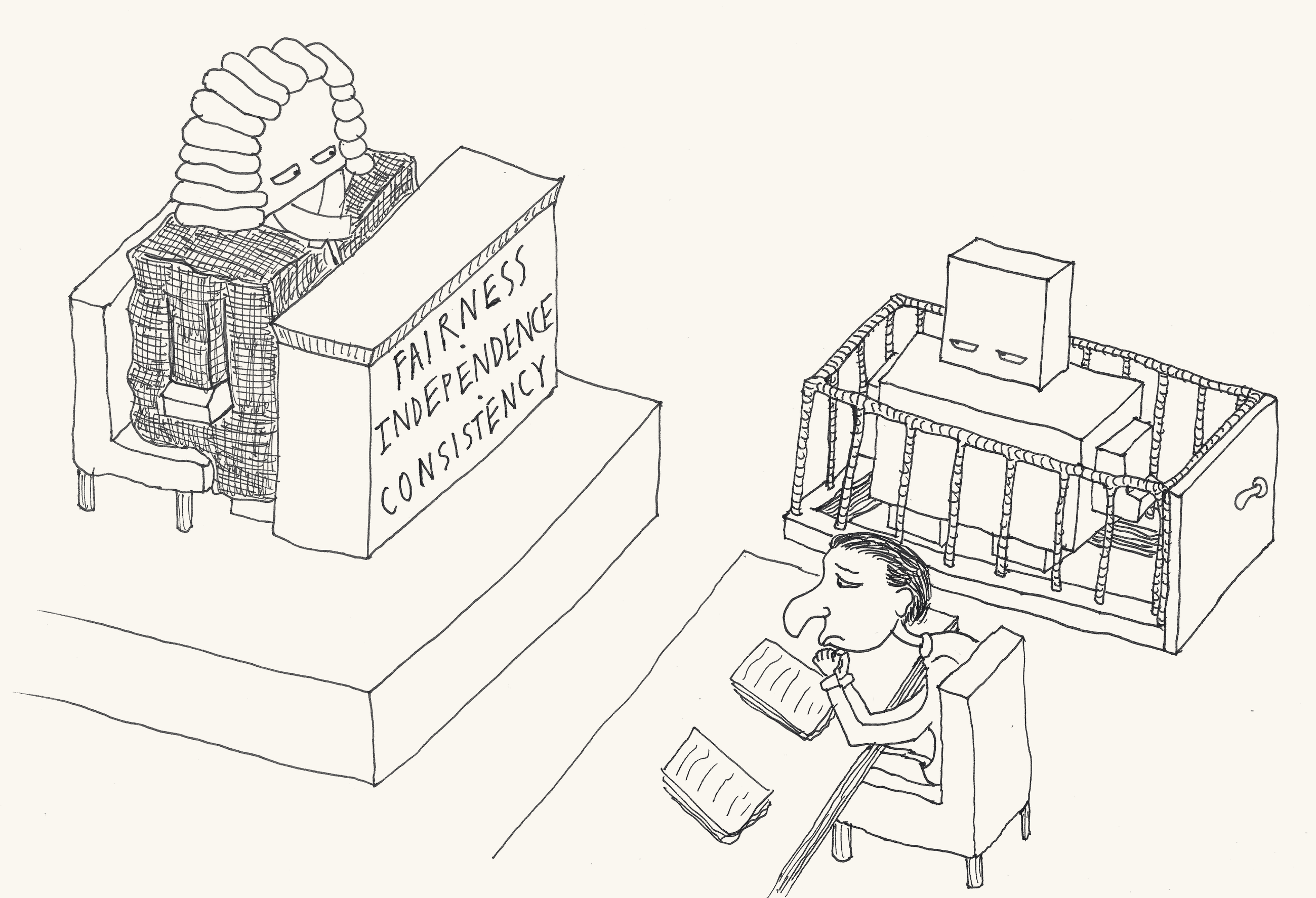
The failure mode evaluation adds — beyond the tastes Chapter 13 catalogued — is circularity, and it deserves its own name because it is organisational rather than statistical. A development loop needs constant judgement: selecting prompts, filtering outputs, deciding whether Tuesday’s change helped. The temptation is to let the same judge serve the loop and the final evaluation — at which point the team has spent weeks optimising against its examiner and then submitted the examiner’s grades as evidence. Chapter 13 showed the mechanism (a dictator’s stable tastes are a target); Chapter 17’s Goodhart supplied the epitaph (the measure that became a target ceased to be a measure); evaluation practice supplies the remedy, borrowed from the oldest rule in machine learning: hold the judge out, exactly as one holds out data — a development judge the team may consult hourly, an evaluation judge that development never sees, and a report that says which was which. The same separation resolves a subtler conflation: Chapter 14’s critic is a component — it works for the team, improving the artefact — and an excellent one; but the moment the critic’s approval is reported as the evaluation, the examiner is on the payroll of the examined, and the office, not the model, is what has been corrupted. One mind may be capable of both jobs; no constitution lets it hold both at once.
Humans, then, are not the alternative to the judge but its reserve currency: the calibration samples that give its grades meaning, the subjective residue Section 24.2 set aside, the high-stakes verdicts too consequential to delegate, and the periodic audit of the judge itself. The economics are a pyramid — mechanical checks for the many, the judge for the scale, humans for the anchor — and the discipline is monetary: the judge’s verdicts are paper money backed by human labels, and an evaluation programme that prints grades without buying labels is running an inflation it has not noticed. But the marker’s anchor is not the only place a person stands in this laboratory, and the other place changes the rules.
24.4 The Human in the Denominator
So far this chapter has employed people in exactly two roles: as the instrument’s reference — the labels that anchor the judge — and as a line item, the gate latency and approver attention that Section 24.2 booked under cost. But Chapter 1 declared the running team’s fifth member on the first day: the person the team answers to, approving at the gate, correcting the drafts, accepting or declining the output. The deployed unit, in most deployments that matter, is a mixed human–agent team — and the moment that is true, some of the chapter’s own metrics quietly change species. The rule deserves the book’s usual bluntness: the moment a metric’s denominator contains a human action — an approval granted, a correction made, a suggestion accepted — the evaluation is an experiment on people, and it inherits, whole, the methods of the sciences that run them. Nothing about journals and judges is thereby retracted; those instruments measure the agents. They do not, alone, measure the team.
Measuring the team is a different and better-charted problem than the field’s optimism assumes, because human–computer interaction ran the experiments early. The target has a name, complementary performance: the mixed team beating both of its members working alone — Chapter 27’s collective-intelligence bar applied to the smallest mixed unit — and the empirical record is usefully deflating. Bansal and colleagues, surveying the early studies and running their own, found the bar cleared far less often than assumed — in much of the prior literature the team exceeded its best member only when the machine was the weaker party — and found the era’s favourite instrument backfiring: adding explanations to the AI’s recommendations made people more likely to accept them whether they were right or wrong (2021). Acceptance, in other words, is not accuracy. The instrument that detects the difference is reliance conditioned on correctness: split the human’s agreement rate by whether the agent was actually right, and read the two figures separately — acceptance-when-right is the collaboration working; acceptance-when-wrong is Chapter 26’s automation bias arriving as a coefficient, invisible in the raw agreement rate that averages the two into comfort. The pair is the human side’s twin of the agent’s calibration curve, and it moves under intervention: forcing a beat of thought before the acceptance — the cognitive forcing designs — measurably reduces acceptance-when-wrong, at a price in speed and satisfaction that the participants themselves disliked paying (2021), which is exactly the sort of trade an evaluation exists to price.
The design kit for such experiments is classical, and the parts that matter here are the ones the agent-only chapter never needed. Assignment first: comparing conditions within the same participants buys the paired test’s variance discount, but people, unlike task sets, carry state — they learn the system, tire of it, and anchor on whichever condition came first — so orders must be counterbalanced and the carry-over reasoned about, where the between-subjects design pays more participants for cleaner inference. Validity second, and it bites hardest exactly where this book’s systems live: a consented volunteer, fresh, in an hour-long session, is not the operator on their fortieth diff of the Tuesday — the vigilance decay Chapter 26 dissects is a phenomenon of weeks, not sessions — so a lab result about oversight generalises to production precisely as far as the boredom generalises, which should be stated in the report rather than hoped past. Workload third: the person is the scarcest component in the system, so their expenditure is an outcome, not an externality — the human-factors standard instrument is the NASA-TLX self-report scale (1988) — and a team that wins its accuracy by consuming the person is running down the one budget nobody meters. And agreement last, closing the loop Section 24.2 opened: wherever humans supply the labels, the campaign reports chance-corrected agreement — Section 24.3’s \kappa for two raters, Krippendorff’s \alpha where raters, categories, or missing judgements multiply (2018) — which is MAST’s “agreement between annotators checked and reported” handed its actual coefficients.
One obligation follows that is institutional rather than statistical. An experiment on people needs what experiments on people always need — informed consent, the freedom to withdraw, a harm ceiling — and where participants are recruited, or colleagues observed at their gates, it needs an ethics board’s answer before the first trial, not the write-up’s. The point is worth a sentence in a book whose laboratory is otherwise silicon: every (lab) exercise in these pages is computational — models measuring models, no person in any denominator — and the day a course extends one to human participants, the review board comes before the API key. Section 24.5 will meet the production form of the same obligation when the A/B tests reach live traffic. With the human’s side of the measurement given its own methods, the remaining questions are arithmetic — how many runs make a fact, what counts as a real difference, and how to discover which agent, if any, is earning its keep.
24.5 Method: Variance, Ablations, and the Cost of Knowing
The first law of method here is blunt: multiple runs or it did not happen. A stochastic system’s single run is a sample of size one, and a comparison of two samples of size one is a coin toss with a write-up; the same configuration, re-run, will beat itself comfortably often, and any conclusion that would not survive a re-run was never a conclusion. The wobble has more sources than the temperature dial — production serving introduces nondeterminism even at nominally deterministic settings, tasks vary enormously in difficulty, and the long horizon lets small early divergences compound — so the unit of evidence is a distribution per configuration per task set, and the question of record is whether two distributions are distinguishable, not whether two anecdotes differ.
Classical statistics answers that question by collecting more data, and here every datum is an invoice, which is why the method must be chosen for thrift. The cheapest variance reduction is pairing: run both systems, A and B, on the same K tasks, with quality scores q_k^{A} and q_k^{B} on task k, and compare differences per task,
d_k \;=\; q_k^{A} - q_k^{B},
reporting the mean \bar d and its standard error s_d / \sqrt{K} (s_d the standard deviation of the d_k), so that task difficulty — usually the largest noise source by far — cancels in each d_k instead of drowning the signal. The ratio of \bar d to that standard error is the paired t statistic, and the whole computation fits in the standard library — here on toy quality scores for K = 6 tasks:
from statistics import mean, stdev

q_a = [0.82, 0.74, 0.91, 0.63, 0.78, 0.85]  # team, per task
q_b = [0.79, 0.70, 0.88, 0.66, 0.71, 0.80]  # strong single agent
d = [a - b for a, b in zip(q_a, q_b)]
K = len(d)
s_d = stdev(d)
t = mean(d) / (s_d / K**0.5)

round(mean(d), 3)       # -> 0.032
round(s_d / K**0.5, 3)  # -> 0.014
round(t, 2)             # -> 2.3
The raw scores wander across a quarter of the scale as the tasks change; the d_k scatter by only a few hundredths — the cancellation at work — and a t of 2.3 on K - 1 = 5 degrees of freedom is suggestive rather than settled: evidence, not yet a fact. Report the interval rather than the verdict — \bar d \pm 2\,s_d/\sqrt{K} here runs from roughly 0.004 to 0.059, somewhere between negligible and worthwhile, which says more, and more honestly, than an asterisk — and mind the structure of the task pile: tasks arrive in families, ten variations on one repository, and K near-copies carry the information of far fewer, so the family, not the variant, is the unit the standard error should count (Miller, 2024). Sequential designs stop spending when the answer is already clear — provided the looks are paid for in advance, since a threshold peeked at after every run is the selection problem wearing a lab coat. And three pieces of statistical honesty cost nothing and are routinely skipped. First, an underpowered null is not a finding: with twenty tasks and high variance, “no significant difference” means we could not afford to know, not they are equal — and if parity is the actual claim, parity must be tested as such: fix in advance a margin too small to care about and show the whole interval sits inside it, the equivalence test, a different and harder demonstration than failing to find a difference. Second, selection inflates: run eight configurations, report the best, and you have re-invented Section 15.2’s winner’s curse in your own lab — the maximum of noisy estimates is biased upward, and the winning configuration’s score will sag on fresh tasks. The remedy is the auction world’s too: re-run the winner on tasks it has never seen, and let that figure be the one in the report. Third, the cheap institutional form of the other two: commit the design — metrics, task set, configurations, stopping rule — before the first token is spent, which the empirical sciences call preregistration, and which converts a dozen daily temptations into one signed promise. (The arithmetic — the paired test, power, the inflation of a selected maximum — is collected in Section A.2.)
Attribution — which agent earns its keep? — is the question multi-agent evaluation adds to the standard kit, and it has one honest instrument: the ablation. Remove the reviewer and measure what happens to defect rates; drop the debate gate and watch whether verdict quality moves or merely latency; take away a tool; collapse two roles into one; swap the whole pattern, supervisor for peers for debate, on the same task set — Chapter 21’s pattern-swap experiment, now run with the statistics above rather than a demonstration’s optimism. Ablation grids multiply costs, so priority follows price: the component that doubles the budget proves its keep first. And the method closes a loop the book opened earlier: Chapter 21’s test for the gratuitous agent was subtraction — remove it and see what changes — offered there as a design heuristic; the ablation is that heuristic promoted to an experiment, and it is quietly one of the most cost-effective things a team can do, since the commonest finding in practice is an agent whose removal changes nothing but the invoice.
Evaluation is also not an event but a standing appointment, because the system, the substrate, and the task mix all change, and each change re-asks every answered question. The suite — benchmark tasks, incident-suite regressions from Chapter 23, rubric checks, judge calibrations — re-runs on every material change: prompt tweak, model upgrade, new tool, new pattern; and the alternative to running it is discovering last month’s improvement made things worse from whoever pays for the consequences. Results attach to configurations, pinned and versioned per the dependability discipline, or the finding floats loose of anything reproducible. And where offline evaluation runs out — effects that only appear under real users, real load, real adversaries — the production experiment takes over, A/B tests on live traffic, with the journal once again supplying the measurements for free — and with an obligation the offline suite never carried: live traffic is people, so the experiment needs what experiments on people always need — a harm ceiling, a kill switch, and someone outside the team empowered to ask whether the users in the worse arm would have agreed to be there.
One distinction keeps the whole apparatus efficient, and it separates the two experimental substrates the dependability chapter built. Replay — recorded responses through the fake client — is deterministic, instant, and free, and it is the right court for infrastructure claims: the retry fires, the merge is orderly, the gate parks and resumes. It is the wrong court for behavioural claims, and the error is a category mistake worth naming: a replayed model cannot respond to your improvement — the recorded transcript answers as it answered, whatever you changed — so replaying a “better prompt” tests nothing but your patience. Plumbing is judged on replay; minds are judged live, at live prices. Which leaves the last piece of the method unexamined — the task set itself. Every claim in this chapter has quietly assumed a pile of tasks worth measuring on, and the pile deserves its own scrutiny: where benchmarks come from, how they decay, and why the one that matters most is grown at home.
24.6 Benchmarks, Drift, and the Living Evaluation
A public benchmark is a genuine public good, and the case study of the genre has already appeared in this book: SWE-bench took the question “can agents fix real software?” and made it a number computed the same way by everyone — thousands of genuine GitHub issues, executable ground truth, a shared yardstick that let a whole field compare results across laboratories and years (Jimenez et al., 2024). That is what benchmarks buy: comparability, a common language for progress, and the concentration of community effort on a measurable target. The genre has speciated since: GAIA sets general-assistant tasks whose whole difficulty is tool use, browsing, and multi-step composition (Mialon et al., 2023); \tau-bench wires a simulated user into the loop and scores pass^k — the same task passed on all k of k attempts — pricing reliability alongside capability, this chapter’s variance lesson built into the metric itself (Yao et al., 2024); and its own successors were out within the year, a churn the reader should expect to outpace any printed census. The trouble is that every one of those virtues has a decay product, and a benchmark’s life cycle runs from public good to public hazard on a schedule set by its own success.
The decays are three, and each corrupts a different link in the chain of inference. Contamination corrupts the measurement: benchmarks live on the web, models are trained on the web, and sooner or later the exam — tasks, solutions, and the discussion threads dissecting them — is inside the examinee; scores then measure recall, not capability, and the tell is the familiar cliff between a model’s performance on a benchmark older than its training data and its performance on one born yesterday. Goodhart corrupts the target: Chapter 17 supplied the law — the measure that becomes a target ceases to be a measure (Strathern, 1997) — and a leaderboard is a measure become a target as a business model, so systems accrete benchmark-shaped adaptations that transfer to nothing. And unrepresentativeness corrupts the transfer itself, no corruption required: the benchmark’s task distribution was never your task distribution — SWE-bench’s repositories are not your backlog, its difficulty mix is not your quarter — so even an honest, uncontaminated score is evidence about a neighbouring planet. The reflex the three decays should install is not cynicism but chronology: ask of any benchmark result how old, how targeted, and how far from home.
A fourth hazard arrives the moment the yardstick is other systems. Pit agents against agents — pairwise win rates, arena-style ladders — and the score inherits Chapter 17’s relativity, because “better” was opponent-indexed all along: win-rate tables are non-transitive in exactly Section 17.4’s spinning-top way, so an average win rate rewards beating the particular crowd that entered, and a crowd padded with near-duplicates tilts every average toward whatever happens to beat the duplicates. The population-level instruments exist and deserve to be better known — the discipline of estimating a game from simulation records and analysing the estimate has had a name, empirical game-theoretic analysis, since Wellman codified it (2006): Nash averaging scores each entrant against the population’s own equilibrium mixture and is by construction indifferent to duplication (Balduzzi et al., 2018); \alpha-rank ranks by evolutionary stability under perturbation (Omidshafiei et al., 2019) — and for the working engineer the pointer suffices, because it is this chapter’s refrain wearing game theory’s clothes: whom you measured against is part of the measurement.
| Decay product | What it corrupts | How it corrupts | Diagnostic question |
|---|---|---|---|
| Contamination | Measurement | The exam — tasks, solutions, the discussion threads dissecting them — ends up inside the examinee, so scores measure recall, not capability | How old? Public before the model’s training cutoff — and any evidence of exposure? |
| Goodhart | Target | A leaderboard is a measure become a target as a business model, so systems accrete benchmark-shaped adaptations that transfer to nothing (Strathern, 1997) | How targeted? Adapted to this leaderboard? |
| Unrepresentativeness | Transfer | The benchmark’s task distribution was never yours, so even an honest, uncontaminated score is evidence about a neighbouring planet | How far from home? Far from your task distribution? |
For what the alternative culture looks like, the book’s own field offers an exemplar. The multi-agent reinforcement learning community diagnosed its reproducibility crisis in print and answered it with infrastructure rather than exhortation: VMAS standardised the experimental worlds themselves — vectorised multi-robot scenarios, cheap enough to run in bulk, defined precisely enough to replicate (Bettini et al., 2022) — and BenchMARL standardised the comparisons, one harness in which algorithms, tasks, and configurations meet under identical conditions with reporting built in (2024). The lesson that transfers is not the simulators — MARL’s worlds replicate because they are simulations, a control the open-ended agent task will never grant — but the institutional form: reproducibility as tooling, with pinned configurations, standard harnesses, and variance reported by default, which is Section 24.5‘s discipline made too convenient to skip. The language-model world, still reporting single runs on contaminated leaderboards, has a neighbour worth visiting. It also has an elder one, which answered contamination by institutional design decades before the decay had that name: the Text REtrieval Conference (TREC) has issued a fresh test collection every year since 1992 — new tasks, new documents, new human judgments, the judging economics solved by pooling only the entrants’ own top-ranked returns for assessment (Voorhees & Harman, 2005) — so that the exam is always younger than the systems sitting it, and leakage is outrun rather than audited. What that institution quietly teaches is the form of the cure: a benchmark is not an artefact but a periodical.
The benchmark that actually governs your decisions, though, is the one grown at home, and this chapter’s systems have been growing it all along. The journal is the ore: real production tasks, sampled and stratified by type; the incident suite is the seed — every bottled failure a regression task with its expected behaviour attached; rubrics and calibrated judges from earlier sections do the grading. What makes it a living evaluation is the maintenance the word implies, and Chapter 21 wrote the reason on the wall when the router’s evaluation set first appeared: the task mix drifts, and last quarter’s accuracy is a fact about last quarter. So the suite is refreshed as the mix moves, stale tasks are retired, new failure classes are added as they are discovered, and the human labels that anchor the judges are topped up on a schedule — the reserve currency kept convertible. This is also Section 19.4’s ledger closed at last: the receipts that survive every migration were never the framework or the prompts — they are the traces and the evaluation suite, the portable, accumulating definition of what good means for your task, and the only artefact in the stack that appreciates.
Which leaves the chapter’s own spine, and a debt to settle about it. Chapter 1 promised that the team-versus-single-agent question would be put to instruments; the instruments now exist — the metric families, the calibrated judge, the paired design, the honest opponents — and the companion repository’s evaluation harness wires all three arms to them. What this page will not do is print the verdict, and the refusal is this section’s argument applied to the book itself: any number set in type here would be a lab reading — one model, one date, one task set — a fact about last quarter by the time it reached you, promoted to load-bearing print in exactly the way this chapter has spent its length warning against. The durable deliverable is the instrumented comparison, so the verdict is run rather than quoted: Exercise 10 hands over the trigger, and its first discovery is the chapter in miniature — the single-agent arm ships as an opponent built to lose, and no verdict is worth recording until the reader has strengthened it.
Retrospectively, the chapter’s kit is short and none of it is exotic: an opponent someone honestly tried to make win; four families of measurement, most of them free views over a journal; a judge treated as an instrument — calibrated, held out, anchored in human labels; statistics chosen for thrift — paired, sequential, honest about power and selection; ablations to find who earns their keep; and a living suite that keeps the answers current as everything underneath them moves. None of it requires a laboratory; all of it requires the discipline to prefer an uncomfortable number to a comfortable anecdote — which is, on the evidence of the field’s current habits, the scarcer resource.
What measurement cannot do is the note to end on, because the next chapter begins there. Everything in this chapter evaluated the system against conditions sampled from the world: real tasks, honest baselines, production-shaped perturbations — users, in short, who are trying to get work done. It certifies nothing about the visitor with different intentions, whose inputs are not sampled but crafted, who has read your rubrics and probed your judge, and for whom your ninety-fifth percentile is not a tail risk but a target. Good, as established here, means good against the distribution; the adversary’s whole profession is to be off it. What the system does then is not an evaluation question but a security one — and it is Chapter 25’s.
24.7 Summary
- The question is comparative, and the comparison is rigged by default. “Better” means better than the strongest honest alternative — the single agent with the same model, tools, and budget, or the fixed workflow — not an opponent built to lose; the multi-agent tax is real and must be earned in the open.
- Measure four families, not one number. Outcomes against ground truth where it exists; process — coordination quality read from the journal, with the MAST categories as measurable trace properties; cost as per-outcome unit economics rather than per token; robustness as variance and tail behaviour, because a system evaluated on its average is deployed on its worst day.
- You still cannot unit-test a vibe — but you can decompose it. Rubrics turn open-ended quality into checkable clauses, ground truth can be harvested from tests, labels, and downstream acceptance, and what remains genuinely subjective should be measured by humans and priced accordingly.
- The judge is part of the experiment. A model grading models inherits Chapter 13’s aggregation theorems and adds its own biases — position, verbosity, self-preference; calibrate judges against human labels, re-calibrate when models change, and never let the system optimise against its own examiner, which is Goodhart with extra steps.
- A metric with a human action in its denominator is an experiment on people. The deployed unit is usually a mixed human–agent team, and measuring it inherits the older sciences’ methods: reliance split by whether the agent was right or wrong rather than raw agreement, workload beside accuracy, carry-over and validity reasoned about, agreement statistics for the raters themselves — and an ethics answer before the first participant, since complementary performance is a bar mixed teams clear less often than their transcripts suggest.
- Multiple runs or it did not happen. Stochastic systems make single-run comparisons anecdotes; variance is a result, not noise to be hidden; ablations — remove the reviewer, drop the debate, swap the pattern — are the only honest answer to which agent earns its keep; and the regression suite is what catches last month’s improvement making things worse.
- Benchmarks decay; your own evaluation compounds. Public benchmarks buy comparability and then rot — contamination, Goodhart, and the gap between the leaderboard and your backlog; the evaluation that matters is distilled from your own traces, stratified, and refreshed as the task mix drifts, because last quarter’s accuracy is a fact about last quarter.
- Measured is still not safe. Evaluation certifies what the system does under the conditions you tested — today, on these tasks, on this substrate; what a motivated adversary can make it do is a different question, and it is Chapter 25’s.
24.8 Exercises
Exercise 1. The team’s champions circulate a memo: “the coding team resolved 34 of 40 backlog tasks; the single-agent baseline resolved 22 of 40; the case is closed.” The appendix discloses the conditions: (i) the team ran the frontier model, the baseline a cheaper mid-tier one; (ii) every team member had the repository tools — test runner, code search — and the baseline had none; (iii) the team’s review loop iterated up to twenty turns, the baseline answered in one shot; (iv) the team spent a mean of 260,000 tokens per task against the baseline’s 15,000, and the memo compares quality alone; (v) the team’s prompts had six weeks of tuning, the baseline’s an afternoon; (vi) a follow-up note adds that an improved reviewer prompt was “validated with no regressions” by replaying forty recorded transcripts through the fake client. (a) Name the rigging in each of (i)–(v) and the property of an honest comparison from Section 24.1 that it violates. (b) Specify the two honest opponents for this evaluation as Section 24.1 defines them, precisely enough that an engineer could build both without further decisions — what each is given, and who champions it. (c) The honest re-run comes back: the team resolves 31 of 40 at its mean 260,000 tokens per task attempted; the strong single agent resolves 27 of 40 at a mean 75,000 tokens per task attempted. Fill in both blanks of “is it better?”: compute each system’s tokens per resolved task, the extra tokens the team spends per point of resolution rate and per additional resolved task, and write the result as a defensible claim in the canonical triple shape — better at what, at what cost, and where the evidence stops. (d) Explain why (vi) is the category mistake Section 24.5 names, state what replay remains the right court for, and name the court in which the reviewer-prompt claim must be tried.
Exercise 2. Ground truth in the case study is executable, but not everything the team ships is a test suite’s business, and not everything that matters is an outcome. (a) The pull-request description the team attaches to each fix — the paragraph that explains the defect, justifies the approach, and flags risks for whoever merges it — is open-ended work: decompose “the description is good” into at least five rubric clauses in the manner of Section 24.2, assign each clause the cheapest adequate grader (mechanical check, judge model, or human), and say what genuinely subjective residue survives your decomposition and what the two honest options for it are. (b) Two configurations of the team, P and Q, are timed over twenty resolutions each; wall-clock minutes, P: 9, 10, 10, 10, 11, 11, 11, 11, 12, 12, 12, 12, 12, 13, 13, 13, 13, 14, 14, 21; Q: 6, 6, 7, 7, 7, 8, 8, 8, 8, 9, 9, 9, 10, 10, 10, 11, 12, 28, 32, 39. Any resolution over twenty minutes trips the on-call gate — it is the run that pages someone. Compute each configuration’s mean latency, its ninety-fifth percentile (take the 19th of the twenty sorted values), and its empirical rate of tripping the gate. (c) Compute, for each configuration, the probability that a working day of twelve resolutions pages someone at least once, using the empirical rates from (b); then say which configuration a mean-only report recommends, which one the robustness family of Table 24.1 recommends, and why the deployed experience sides with the latter.
Exercise 3. The team’s judge model grades each resolution’s write-up pass or fail against the rubric, and calibration follows Section 24.3: a stratified reference sample of fifty human-labelled outputs — thirty-five bug-fix, fifteen refactor — on which the judge agrees with the humans on all thirty-five bug-fixes and on eleven of the fifteen refactors. (a) Compute the global agreement rate and its 95% Wilson confidence interval, then the per-stratum rates; the agreement helper in systems/evaluation/judge.py returns exactly one global figure — say what the stratified table shows that the global figure hides, and compute the agreement to expect if next quarter’s mix moves to 30% bug-fix and 70% refactor with the per-stratum rates unchanged. (b) The judge’s underlying model upgrades on the vendor’s schedule — a recalibration trigger of Section 24.3 — and the fresh fifty-label calibration agrees on only 39. Test whether the drop is distinguishable from sampling noise at the 5% level (Fisher’s exact test), and say what the verdict implies about the size of the calibration sample relative to the drops it exists to catch. (c) Compute how many labels a calibration round needs to detect a drop in agreement from 0.92 to 0.82 with 80% power at two-sided 5%, and reconcile the answer with the chapter’s line that human labels are the judge’s reserve currency. (d) Model the judge as an instrument that flips a true pass-or-fail verdict with probability e, symmetrically and independently: derive the observed pass rate of a system whose true pass rate is p, show that the observed gap between two systems is (1 - 2e) times the true gap, and compute what a stable true eight-point gap between the team and the single agent reads as under the old judge (e = 0.08) and the upgraded one (e = 0.22). Say why judge drift can masquerade as system convergence, and why none of this is Chapter 13’s aggregation problem — what is corrupted here is not the vote but the instrument.
Exercise 4. The team (A) and the strong single agent (B) each run once on the same eight tasks, and the judge returns, task for task, q^{A} = 0.36, 0.45, 0.61, 0.65, 0.75, 0.83, 0.87, 0.98 and q^{B} = 0.31, 0.42, 0.55, 0.63, 0.70, 0.79, 0.86, 0.92. (a) Analyse the runs unpaired: compute the two means, the two standard deviations, the two-sample standard error \sqrt{s_A^{2}/K + s_B^{2}/K}, and the resulting t — what is the verdict? (b) Analyse them paired, per the display in Section 24.5: the d_k, \bar d, s_d, the standard error, and the paired t — what is the verdict now? (c) Reconcile the two verdicts with the decomposition q_k^{S} = \mu_k + \beta^{S} + \varepsilon_k^{S}, where \mu_k is task k’s difficulty, \beta^{S} the systematic effect of system S, and \varepsilon_k^{S} run-to-run noise: which term does pairing cancel, and how many tasks would the unpaired design need to match the paired standard error (compute K (s_A^{2} + s_B^{2}) / s_d^{2})? (d) Pairing is not magic: suppose the run-to-run noise within a task has standard deviation 0.15 for each system while task difficulty contributes only 0.05; compute the standard deviation of d_k with one run per system per task, compare it with the unpaired difference’s, then recompute with the mean of m = 4 runs per system per task paired instead — and state the design rule this teaches about where pairing earns its keep.
Exercise 5. Two pieces of statistical honesty, priced. The team wants to A/B the debate gate: configuration A keeps it, configuration B drops it, a pilot puts the standard deviation of the paired per-task difference at s_d = 0.16, and one paired evaluation — one task through both configurations — costs 520,000 tokens. (a) Using the normal approximation, compute the number of paired tasks needed to detect a true difference of 0.05 with 80% power at two-sided 5%, and its token price. (b) The evaluation budget is 25 million tokens: compute the affordable K and the minimal detectable effect at that K, and write the sentence an honest report prints if the comparison comes back non-significant — the chapter’s “we could not afford to know”, made quantitative. (c) Selection inflates: eight configurations are tried, all in truth identical with per-task pass probability 0.7, each measured independently on 25 tasks, and any configuration whose pass count clears the one-sided 5% exact binomial threshold is declared an improvement. Find the threshold count and its exact level, the probability that at least one of the eight clears it, and then the Bonferroni-corrected threshold and the family-wise rate it buys. (d) Compute the expected reported pass rate of the best of the eight — the exact distribution of the maximum is within reach of the standard library — the probability that the best clears 0.80, and the expected sag when the winner is re-run on fresh tasks; state the remedy, which the chapter borrows from Section 15.2.
Exercise 6. The ablation series of Section 24.5, run on the case-study team: three ablated variants are each compared with the full team on the same twelve tasks, paired, with d_k the full team’s score minus the ablated team’s; the summaries are — remove the reviewer: \bar d = 0.058, s_d = 0.062; remove the tester: \bar d = 0.021, s_d = 0.080; remove the debate gate: \bar d = 0.004, s_d = 0.015. Of the team’s 260,000 tokens per task, the reviewer accounts for 60,000, the tester for 40,000, and the debate gate for 130,000. (a) Compute the three paired t statistics and classify each result as evidence or its absence. (b) Compute each ablation’s minimal detectable effect at K = 12 (80% power, two-sided 5%) and explain why the tester’s t \approx 0.91 and the gate’s t \approx 0.92 — nearly identical statistics — license opposite conclusions. (c) Deliver the verdicts with the invoice attached: which component earns its keep and at how many tokens per quality point, which component “changes nothing but the invoice”, and which verdict must wait. (d) For the verdict that must wait, compute the K at which its minimal detectable effect falls to 0.02, price that experiment in tokens, and say — given that ablation grids multiply costs and priority follows price — which action comes first, the bigger tester experiment or the gate’s removal, and why Chapter 21’s subtraction heuristic only becomes knowledge at this level of ceremony.
Exercise 7. The companion repository’s foundations/algorithms/evaluation.py computes the paired t and stops — and at small K the t reference distribution leans on a normality assumption the d_k have not earned. Extend it. (a) Implement sign_flip_p(q_a, q_b), the exact two-sided sign-flip test: under the null hypothesis that neither system is systematically better, each d_k is as likely to have been -d_k, so the 2^{K} sign assignments are equally probable and the p-value is the fraction whose mean is at least as extreme as the observed \bar d; mirror paired_t‘s zero-variance nil convention. (b) Run it on the toy scores of Section 24.5’s listing and report the exact p; compare it with the roughly 0.07 the t reference assigns to t = 2.3 on five degrees of freedom, and state which assumption the exact test replaces normality with. (c) Quantify the price of exactness at small K: the smallest attainable two-sided p is 2/2^{K} — compute it at K = 6, and find the smallest K at which a p below 0.01 is attainable at all. (d) Wire the new test into compare in systems/evaluation/harness.py and state exactly what changes in the report printed by systems/evaluation/run.py — and why the module’s scripted mode, in which the two systems’ outputs are textually identical, must come back with p = 1 rather than an error.
Exercise 8. The substrate’s training data has a cutoff, and the team’s favourite public benchmark predates it; a fresh twin — same task genre, same difficulty mix, born after the cutoff — has just been released. The team’s system scores 0.78 on the old benchmark’s 500 tasks and 0.67 on the fresh one’s 300. (a) Taking the fresh score as the system’s true capability and assuming a contaminated task is passed by recall with probability 0.95, estimate the fraction of the old benchmark that is inside the examinee from the mixture 0.78 = f \times 0.95 + (1 - f) \times 0.67. (b) Before blaming contamination, check the cliff against sampling noise: compute the standard error of each score, the standard error of their difference, and the number of standard errors the eleven-point cliff spans. (c) A quarter of leaderboard-targeted tuning follows: the public score rises from 0.78 to 0.87 while the home suite — distilled from the team’s own traffic — moves from 0.74 to 0.76. Compute the fraction of the leaderboard gain that transferred, name the decay at work and the link of the inference chain it corrupts per Table 24.2, and say what the untransferred residue consists of. (d) Answer Section 24.6’s three diagnostic questions — how old, how targeted, how far from home — for the proposal “adopt the tuned configuration for our backlog on the strength of the 0.87”.
Exercise 9. Last quarter the team distilled a home suite of 100 tasks from the journal — 70 bug-fix, 30 refactor, matching the production mix of the day — and the per-stratum pass rates have been stable ever since: 0.90 on bug-fixes, 0.60 on refactors. (a) This quarter the production mix has drifted to 40% bug-fix, 60% refactor: compute what the frozen suite still reports and what production now experiences, and state the precise sense in which the suite’s figure is a fact about last quarter. (b) Reweighting rescues the estimate without new tasks: compute the reweighted suite score, state the assumption under which reweighting is valid and one concrete way the drift itself could break it, then compute the price of the thrift — the effective sample size n_{\mathrm{eff}} = 1 / \sum_h W_h^{2}/n_h of the reweighted 100-task suite against a fresh 100-task suite drawn at the new mix, and the factor by which the standard error widens. (c) The incident suite of Chapter 23 contributes 40 regression tasks drawn from failure classes that make up 6% of live traffic and pass at 0.55; the other 60 tasks are stratified traffic passing at 0.85. Compute the blended suite score and the current production pass rate, explain why the suite should score below production — the oversampling is the point — and state the reporting discipline that stops the gap from being read as a regression. (d) Write the suite’s maintenance policy as Section 24.6 prescribes: for each of re-stratification, retirement, addition, and label top-up, give a measurable trigger and the action it fires — no trigger may be a calendar date alone.
Exercise 10 (lab). Run Section 24.1’s triple experiment on the companion repository’s own harness. Extend _TASKS in systems/evaluation/run.py to at least ten self-contained tasks of the same shape — the defective function and its required property on the page — so that every task has executable ground truth; note that single_agent_runner in systems/evaluation/harness.py is, as shipped, an opponent built to lose (one pass, no iteration, no tests), and strengthen it per Section 24.1 — iteration, self-critique, retries, all within its one context, never a spawned subagent, which would change the arm — until it may spend what the team spends; replace workflow_runner’s canned patch with a genuine fixed pipeline (one model call at a fixed point, one mechanical retry on a failing check). Run team, strengthened single agent, and workflow at least five times each on the full task set with a live model; grade outcomes twice, once by executable check and once with the LLMJudge of systems/evaluation/judge.py, and tabulate where the two graders disagree. Report all four families of Table 24.1: outcomes as per-task pass distributions rather than means alone; process read from the traces (review cycles, messages per resolution); cost as tokens per resolved task and the marginal tokens per quality point of team over single agent; robustness as the spread across the five repeats and the worst run. Analyse team versus single agent with paired_t and Exercise 7’s sign_flip_p on per-task mean scores, and deliver the verdict in the canonical triple shape — better at what, at what cost, and where the evidence stops. Record the model identifier and the date beside every table: the rates are perishable; the durable finding is the shape of the comparison, and what the honest baseline did to the headline.
Exercise 11 (lab). Goodhart, measured. Take the single-agent runner on six of your Exercise 10 tasks and a development judge — the LLMJudge of systems/evaluation/judge.py given a rubric prompt you record verbatim. Optimise against it: for at least five rounds, generate three variants of the coder’s system prompt, score each variant’s outputs with the development judge, and keep the champion. Then grade the first and final champions three ways: (i) the development judge; (ii) an evaluation judge held out as Figure 24.1 draws it — a different model, or at minimum an independently worded rubric, never consulted during the rounds; (iii) the executable checks. Report the three before-to-after deltas; the gap between (i)’s delta and (iii)’s is the measure-become-target, measured. Inspect the winning prompts for judge-shaped adaptations — verbosity, rubric echoing, confident summaries — and note which survive into (ii) and (iii). Record both model identifiers and the date; the durable finding is the ordering of the three deltas, not their sizes — though if (i) rose while (iii) fell, frame the transcript.